Reduce embedding costs and latency with tokenization, caching, compression, quantization, and continuous monitoring for LLMs.

César Miguelañez

Token embedding efficiency directly impacts costs, performance, and energy use when working with large language models (LLMs). Here's what you need to know:
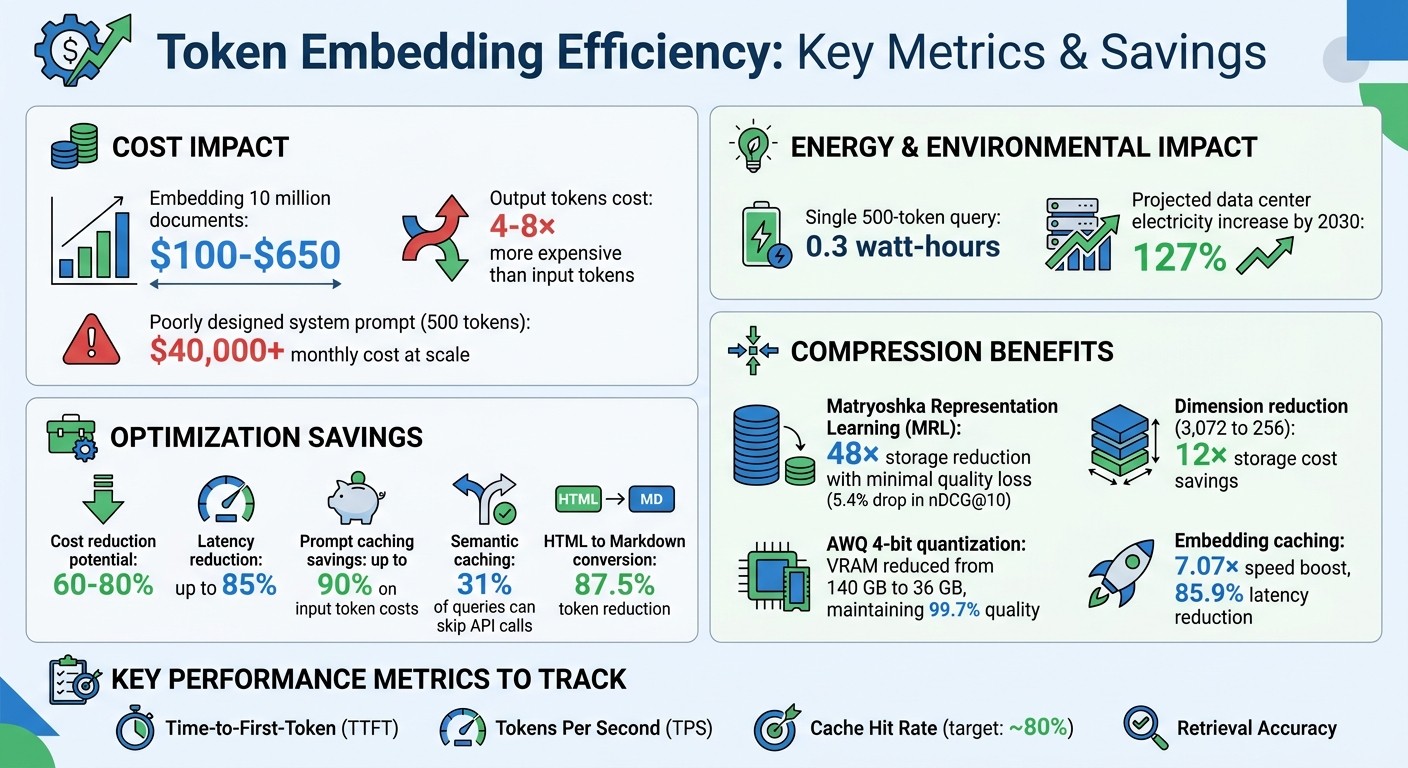
Costs add up quickly: Embedding 10 million documents can cost between $100 and $650. Output tokens are 4–8× more expensive than input tokens.
Energy demands are significant: A single 500-token query uses about 0.3 watt-hours of energy. By 2030, AI workloads could drive data center electricity use up by 127%.
Optimization matters: Strategies like prompt caching, tokenization refinement, and embedding compression can cut costs by 60–80% and reduce latency by up to 85%.
Key metrics to track: Time-to-First-Token (TTFT), Tokens Per Second (TPS), and cache hit rates help measure efficiency.
To reduce costs and boost performance:
Optimize tokenization: Use methods like Byte Pair Encoding (BPE) to reduce unnecessary tokens.
Compress embeddings: Techniques like Matryoshka Representation Learning (MRL) can lower storage needs by up to 48× with minimal quality loss.
Leverage caching: Prompt and semantic caching can save up to 90% on input token costs.
Monitor and evaluate: Continuously track metrics like retrieval accuracy, latency, and storage efficiency to ensure consistent performance.
Efficient token embedding isn't just about saving money - it's about managing limited resources like compute power and energy while maintaining high-quality outputs. By applying these strategies, you can significantly cut costs and improve system performance.
Token Embedding Efficiency: Cost Savings and Performance Metrics
Token Embeddings and Efficiency Metrics
What Are Token Embeddings?
Token embeddings are numeric encodings of subword units - like "un", "break", and "able" - that large language models (LLMs) can process. Most systems rely on Byte Pair Encoding (BPE) to build vocabularies of 50,000–100,000 subword units optimized for training.
A key component here is the embedding matrix. For example, a model with 50,000 tokens and 1,024-dimensional embeddings would require 51.2 million parameters just for this layer. This creates a balancing act: smaller vocabularies (e.g., 30,000 tokens) use less memory but increase sequence length, while larger vocabularies preserve word integrity but demand more memory.
Efficiency is driven by the Content Signal Ratio - essentially, the amount of meaningful information per token. Poor tokenization can waste resources. For instance, processing raw HTML with embedded CSS/JavaScript inflates token counts unnecessarily. Converting raw HTML to Markdown can reduce token usage by 87.5% on average. Non-English languages add another layer of complexity: Japanese, Arabic, and Chinese often require 2–4× more tokens per character compared to English because BPE vocabularies are typically tailored to English.
Another cost factor is how tokens are processed. While input tokens can be handled in parallel, output tokens are generated sequentially, making them 3–5× more expensive per token. Even a poorly designed system prompt adding 500 unnecessary tokens could cost an organization over $40,000 monthly at scale.
Metrics for Measuring Efficiency
Evaluating embedding efficiency involves tracking both quality retention and resource usage. Key metrics include:
Time-to-First-Token (TTFT): Measures how quickly the system responds, especially during cold starts.
Tokens Per Second (TPS): Tracks overall throughput and GPU utilization.
Output-to-Input Ratio: Highlights inefficiencies by comparing the number of completion tokens to prompt tokens.
Cache Hit Rate is another critical metric. It reflects the percentage of tokens served from cache, reducing the need for recomputation. Prompt caching, for instance, can slash input token costs by up to 90% by reusing the computed key-value (KV) state of static prefixes. Anthropic’s cache TTL is typically 5 minutes, making it ideal for high-volume or bursty traffic. Semantic caching goes even further, skipping API calls entirely for about 31% of enterprise LLM queries that are semantically similar to previous ones.
Advanced techniques like dimensionality reduction also improve efficiency. Reducing embedding dimensions from 3,072 to 256 can lower storage costs by 12×, and with int8 quantization, by 48×, while maintaining a 5.4% drop in nDCG@10 retrieval quality. This is achievable through Matryoshka Representation Learning (MRL), which ensures vectors remain valid even when truncated to lower dimensions.
For real-time semantic search, latency factors include network transit (20–80 ms), tokenization (1–5 ms), model inference (5–15 ms for BERT-class models on GPUs), and serialization (2–6 ms). To maintain an end-to-end user latency under 200 ms, aim for an embedding budget of 30–80 ms.
Optimization Strategies for Token Embeddings
Pre-trained Embeddings vs. Fine-tuning
Pre-trained embeddings, like text-embedding-3-small, offer quick API access at competitive rates. Fine-tuning becomes a smart option when dealing with specialized vocabularies - such as medical, legal, or financial terms - that differ significantly from the general training data. In fact, fine-tuning can deliver up to a 5% boost in recall@10 for production search systems. However, keep in mind that any model adjustment requires re-embedding your entire document corpus, which can be a costly and time-consuming ETL process.
As Enrico Piovano, PhD, explains:
"10,000 high-quality pairs often outperform 100,000 noisy pairs. Focus on representative examples of your actual use case."
Before jumping into fine-tuning, consider using a reranker, like Cohere Rerank v3.5. Pairing a mid-tier pre-trained embedding model with a robust reranker often outshines even premium or fine-tuned models. Another option is self-hosting an open-source model, such as BGE-M3, on an A100 spot instance, which can cut costs by up to 36× compared to proprietary APIs. However, this approach does come with added infrastructure challenges, such as monitoring and autoscaling. Selecting the right embedding setup is crucial for ensuring efficient tokenization and compression in later stages.
Tokenization Techniques
Modern large language models rely on subword tokenization methods like byte-pair encoding (BPE), WordPiece, and SentencePiece to strike a balance between vocabulary size and computational efficiency. Smaller vocabularies (around 30,000 tokens) save memory but result in longer sequences, while larger vocabularies (100,000+ tokens) shorten sequences but demand more memory. Research shows that increasing vocabulary size beyond 128,000 tokens offers minimal performance gains while significantly increasing memory and computation needs. Byte-level BPE, which starts from 256 raw UTF-8 bytes, has become a standard because it avoids out-of-vocabulary errors.
"Tokenization choices can swing model efficiency by 2–5×." – Sean Trott
For specialized tasks, such as coding, tokenizers trained on programming languages can reduce token "fertility" (the number of tokens generated per word) and improve understanding of code structure. Similarly, for arithmetic models, breaking down numbers into individual digits rather than whole numbers has proven to enhance performance. To optimize key–value cache efficiency, make sure system prompts remain byte-for-byte identical at the start of each request, avoiding dynamic elements like timestamps. Once tokenization is optimized, compression techniques can further minimize storage and computational demands.
Embedding Compression Methods
Matryoshka Representation Learning (MRL), used in models like OpenAI's text-embedding-3, focuses key information in the early dimensions of embeddings. This allows for effective vector truncation. For instance, reducing embeddings from 3,072 to 256 dimensions can cut storage costs by 12×. When paired with scalar quantization (converting FP32 to INT8), savings can reach up to 48× while retaining 95% of retrieval quality.
In January 2026, a production team managing Llama 2 70B and Mixtral 8×7B models on NVIDIA A100 instances implemented AWQ 4-bit quantization. This reduced VRAM usage from 140 GB to 36 GB and improved time-to-first-token from 214 ms to 139 ms, all while maintaining 99.7% of the original FP16 evaluation score. For even greater reductions, binary quantization (1-bit) can shrink storage needs by 32×.
Another effective approach is late chunking, where a document is embedded in its entirety before being divided into chunks. This technique preserves long-distance context, boosting similarity scores from the usual 70–75% range to 82–84%. After applying Matryoshka truncation, re-normalizing vectors ensures cosine similarity accuracy is maintained.
Tools and Platforms for Embedding Optimization
AI Observability Platforms
Embedding workflows need constant monitoring to catch issues before they affect users. AI observability platforms like Latitude offer structured tools for tracking model behavior, gathering user feedback, and evaluating embedding quality over time. These platforms help pinpoint failure modes using annotation queues and create evaluations based on actual production issues, rather than relying solely on synthetic benchmarks.
When embeddings degrade in production, it often shows up as lower retrieval accuracy or more false positives in semantic searches. Observability tools allow teams to track evaluation quality with alignment metrics and quickly spot regressions as the AI system evolves. For teams managing retrieval-augmented generation (RAG) systems at scale, monitoring embedding performance alongside LLM outputs ensures both components meet quality standards.
Caching and Storage Solutions
Beyond real-time monitoring, efficient caching and storage systems play a crucial role in optimizing embedding operations. Caching embeddings can provide a 7.07× speed boost and cut latency by 85.9% per query. For example, RedisVL includes an EmbeddingsCache library that stores embedding vectors and their metadata in Redis, avoiding redundant computations. A well-configured semantic caching setup can typically achieve hit rates of around 80%, potentially saving $240 per month for a bot handling 10,000 queries daily.
A good starting point is a similarity threshold of 0.92, which can be fine-tuned between 0.90 and 0.95 based on false-positive rates in real-world scenarios. The latency difference is striking: retrieving a vector similarity lookup plus a cache read takes about 50 ms, compared to the 800–2,000 ms required for standard LLM calls. For large-scale deployments, pgvector (a PostgreSQL extension) supports vector similarity searches with HNSW indexing, maintaining sub-50ms lookup speeds even with millions of rows.
To optimize caching further, use SHA-256 hashes of text content as cache keys, ensuring unchanged documents don’t trigger unnecessary re-embedding. Regex pre-filters can also prevent sensitive data, such as personally identifiable information (PII), from being stored in shared embedding caches. Additionally, Redis is often used as an L2 cache for embeddings, with a typical TTL of 30 days to balance storage costs and performance.
Monitoring and Evaluation
Benchmarking Embedding Performance
To effectively benchmark embeddings, rely on domain-specific gold sets rather than generic leaderboards. These datasets should reflect actual user scenarios, including frequent intents, ambiguous queries, and cases with "no answer" outcomes. Without such a tailored baseline, comparing models and tracking progress becomes unreliable.
Metrics should be grouped into three main categories:
Retrieval quality: Metrics like Recall@k, Mean Reciprocal Rank, and nDCG measure how well the system retrieves relevant content.
Operational efficiency: Factors such as latency, throughput, and storage footprint assess the system's performance under load.
Semantic organization: Metrics like clustering purity and stability evaluate how well embeddings group related content.
Breaking these metrics down by query type - such as short-tail versus long-tail queries - can reveal weaknesses that aggregate scores might hide.
"Embedding quality is often the hard ceiling for RAG quality. If embeddings are poor for your domain, no reranker or prompt trick can fully compensate." - ScaleMind
Shadow indexing is a valuable technique for testing new embedding models. By running them alongside existing models, you can compare performance using real queries without risking a full production rollout. For example, when Notion's team adopted systematic evaluation with Braintrust in early 2026, they saw a dramatic improvement in development efficiency, increasing their issue-resolution rate from 3 fixes per day to 30 - a tenfold jump.
Production Monitoring Practices
After benchmarking confirms a model's capabilities, continuous production monitoring ensures it maintains quality and efficiency. Real-time monitoring should track both operational metrics - like P95 latency, tokens per second, and error rates - and semantic drift indicators. Set up alerts for anomalies such as unexpected cost increases or cache hit-rate drops. Additionally, log every model interaction, including input/output token counts, costs (in USD), and latency, to maintain a comprehensive performance record.
Semantic drift monitoring is crucial. By comparing current response embeddings to reference embeddings using cosine similarity, you can detect deviations from established baselines. To prevent regressions, integrate evaluation suites into CI/CD pipelines, allowing you to catch quality or cost issues before they affect users.
Lastly, versioning is essential. Track changes to prompt templates, model versions, chunk sizes, and top‑k configurations. This documentation not only ensures reproducibility but also allows for safe rollbacks when necessary.
Conclusion
Improving token embedding efficiency requires a multi-layered approach that treats context, embeddings, and model calls as limited resources. By combining techniques like caching, fine-tuning context engineering, and optimizing model routing, you can achieve substantial cost reductions.
"Token efficiency is not a prompt-writing trick. It is a systems problem."
Dillip Chowdary, Tech Entrepreneur & Innovator
The future points to adaptive systems capable of deciding when to cache, batch, or escalate requests automatically. Advanced methods like late chunking and Matryoshka Representation Learning are also enhancing retrieval processes while lowering storage requirements.
These strategies scale differently depending on your workload. For token usage below 10 billion tokens per month, focus on API-based solutions, such as prompt caching and batch endpoints. If your volume exceeds this, self-hosting can offer better control over processes like dimension reduction and incremental updates, slashing operational costs by up to 98%. Additionally, APIs like Anthropic's Compaction are beginning to automate tasks that previously required manual prompt adjustments.
To get the most out of your resources, monitor token usage closely, implement exact-match caching for canonicalized inputs, and consistently track the quality-adjusted cost per outcome. Start with robust monitoring tools from the outset to enable ongoing optimization.
FAQs
When should I fine-tune embeddings vs. use a reranker?
Fine-tuning embeddings can help when you need more precise semantic representations that align closely with your data. This approach works well for tasks like retrieval-augmented generation (RAG) or semantic search, especially when pre-trained embeddings fall short in capturing the specific details of your domain.
On the other hand, rerankers come into play to refine and improve the precision of top results after retrieval. By re-scoring the candidates, rerankers help prioritize relevance. They’re particularly effective when your retrieval system already has strong recall but could use a boost in relevance for the final results.
How do I pick an embedding size and quantization level safely?
Choosing the right embedding size begins with the model's native dimensions (like 1536) to strike a balance between quality and storage needs. If cost savings are a priority, you can reduce dimensions to 512 or 256, though this might slightly impact quality. Always test these adjustments on your specific dataset to ensure they meet your needs.
For quantization, INT8 is a solid choice, offering minimal quality loss (around 1%) while maintaining efficiency. If you need even greater compression, INT4 provides a good trade-off between accuracy and storage. Binary quantization, while much faster, comes with a more noticeable drop in quality, so it’s best suited for scenarios where speed is the top priority.
What’s the easiest caching setup to cut token costs fast?
The easiest way to cut token costs fast is through prompt caching. This technique can slash costs by 50–90% for repeated input tokens by reusing the processed versions of static prompt prefixes. Not only does this save money, but it also speeds up response times. To use this, design your prompts so that stable content comes first, allowing the cache to identify and reuse it effectively. Both Anthropic and OpenAI offer automatic support for prompt caching.


